Introduction
What is Expectation Maximization?
Expectation maximization is a technique used to find maximum likelihood of model parameter when model depends on unobserved or latent variable
History
The EM algorthm was explained and given its name in 1977 paper by A.Dempster,N.Laird and Donald Rubin
They pointed out that the method has been proposed many times in special circumstances by earlier authors, but in 1977 they generalized it and presented as powerful tool for inference.
Basics of probability
a. Probability
If all outcomes are equally likely, the probability or chance of an event happening is:
${\textstyle Probability=} {\displaystyle \frac{Number\,of\,favourable\,cases}{Total\,cases}}$
b. Conditional Probability
It is probability of $A$ given $B$ or $B$ given $A$ i.e. what is probability of $A$ happening given $B$ has already happened and vice versa
${\displaystyle Prob(A\,given\,B)=\frac{Joint\,Prob\,of\,A\,and\,B}{Marginal\,Prob\,of\,B}}$
${\displaystyle P(A|B)=\frac{P(A,B)}{P(B)} }$
c. Joint Probability
Probability of A and B together is called joint probability.
It is product of conditional probability of A given B,times probability of B
${\displaystyle P(A,B)=P(A|B) \cdot P(B)}$
d. Chain Rule
Chain rule permits the calculation of any member of the joint distribution of a set of random variables using only conditional probabilities.
for example with 4 variables, the chain rule produces this product of conditional probabilities:
${\displaystyle \mathrm {P} (A_{4},A_{3},A_{2},A_{1})=\mathrm {P} (A_{4}\mid A_{3},A_{2},A_{1})\cdot \mathrm {P} (A_{3}\mid A_{2},A_{1})\cdot \mathrm {P} (A_{2}\mid A_{1})\cdot \mathrm {P} (A_{1})} \mathrm {P} (A_{4},A_{3},A_{2},A_{1})$
$=\mathrm {P} (A_{4}\mid A_{3},A_{2},A_{1})\cdot \mathrm {P} (A_{3}\mid A_{2},A_{1})\cdot \mathrm {P} (A_{2}\mid A_{1})\cdot \mathrm {P} (A_{1})$
With N variables the same rule will be written as
${\displaystyle \mathrm {P} (A_{n},\ldots ,A_{1})=\mathrm {P} (A_{n}|A_{n-1},\ldots ,A_{1})\cdot \mathrm {P} (A_{n-1},\ldots ,A_{1})} \mathrm {P} (A_{n},\ldots ,A_{1})=\mathrm {P} (A_{n}|A_{n-1},\ldots ,A_{1})\cdot \mathrm {P} (A_{n-1},\ldots ,A_{1})$
A more generalize form will be
${\displaystyle P(\bigcap_{k=1}^n \, A_{k})= \bigcap_{k=1}^n P(A_{k} \vert \prod_{j=1}^{k-1} \,A_{j}) }$
e. Independent rule
If event A and B are independent then joint probability of A and B is given by
${\displaystyle P(A,B)={P}(A) \cdot {P}(B)}$
f. Bayes Rule
When conditional probability of A given B is already given and marginal probability of A and B is known then we can use Bayes Rule to calculate the Probability of B given A
${\displaystyle {P}(B|A)=\frac{P(A|B) \cdot P(B)}{P(A)} }$
g. Discrete Random Variable
If a random variable has only discrete value(e.g. 1,2,4,8,6) from discrete set of numbers then probability mass function P.M.F is used to calculate probability for that variable
i.e. ${\displaystyle p(x)=p_{x}(x)=P(X=x)=p_{i}}$
A set of probability value $p_{i}$ is assigned to each of the value in discrete random variable X
h. Continous Random variable
If random variable has continous values(e.g. 1.234,1.56,2.345) from continuous set of numbers then probability density function P.D.F is used to calculate the probability for that variable
i.e. ${\displaystyle P(a\leq X \leq b)= \int_{a}^{b} f(x) \cdot dx }$
i. Expected value
It is just average or mean ($\mu$) of random variable X
${\displaystyle E(X) = \sum_{i=1}^{\infty} x_{i}p{i} }$
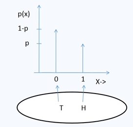
Bernoulli Random Variable
Random variable which takes value 1 with success probability of p and the value 0 with failure probability q=1-p.
It is denoted by ${\displaystyle p_x(x)=\left \{\begin{array}{rcl} \\ p & \mbox if & x=1 \\ 1-p & \mbox if & x=0 \end{array} \right.}$
This can be expressed as
${\displaystyle p_x(x)=\begin{array} \\ p^{x} (1-p)^{1-x} & \mbox x \in \{0,1\} \end{array}}$
Example: Outcome space of random experiment of tossing a coin with success as head and failure as tail
i.i.d. (Independent and identically distributed)
A variable is i.i.d if it is drawn independently from same distribution
A model that includes i.i.d random variable is called i.i.d model with parameter $\theta$
Let $X=\{X_1,X_2,X_3....X_n\}$ be independent and identically distributed random variable then $p(X)=p(X_1,X_2,X_3....X_n)=p(X_1)\cdot p(X_2) \cdot p(X_3) ....p(X_n)$
Expectation Maximization Algorithm
The EM algorithm is an efficient iterative procedure to compute the Maximum Likelihood (ML) estimate in the presence of missing or hidden data. In ML estimation, we wish to estimate the model parameter(s) for which the observed data are the most likely.
Each iteration of the EM algorithm consists of two processes:
The E-step,and the M-step.
In the expectation, or E-step, the missing data are estimated given the observed data and current estimate of the model parameters. This is achieved using the conditional expectation, explaining the choice of terminology.
In the M-step, the likelihood function is maximized under the assumption that the missing data are known. The estimate of the missing data from the E-step are used in lieu of the actual missing data.
Convergence is assured since the algorithm is guaranteed to increase the likelihood at each iteration.
Example
We will understand EM using below example
1) Estimating mean and std-dev for two sample groups
Suppose we are given two sets of samples, red and blue, drawn from two different normal distributions. Our goal will be to find the mean and standard deviation for each group of points.
import numpy as np

np.random.seed(110) # for reproducible results

# set the parameters for red and blue distributions we will draw from
red_mean = 3
red_std = 0.8

blue_mean = 7
blue_std = 2

# draw 20 samples from each normal distribution
red = np.random.normal(red_mean, red_std, size=20)
blue = np.random.normal(blue_mean, blue_std, size=20)

both_colours = np.sort(np.concatenate((red, blue))) # array with every sample point (for later use)

%matplotlib inline

import matplotlib.pyplot as plt

plt.rcParams['figure.figsize'] = (15, 2)

plt.plot(red, np.zeros_like(red), '.', color='r', markersize=10);
plt.plot(blue, np.zeros_like(blue), '.', color='b', markersize=10);
plt.title(r'Distribution of red and blue points (known colours)', fontsize=17);
plt.yticks([]);

Visually from the plot we can say what is mean and std-dev for red and blue points, but let's confirm what is mean and std-dev for each group
what is mean and std-dev of two groups?
print "mean for red : "+str(np.mean(red))
print "std-dev for red : "+str(np.std(red))
print "mean for blue : "+str(np.mean(blue))
print "std-dev for blue : "+str(np.std(blue))
Hidden colors
Now suppose these colors were actually hidden and we can see only black color as output
plt.rcParams['figure.figsize'] = (15, 2)

plt.plot(both_colours, np.zeros_like(both_colours), '.', color='black', markersize=10);
plt.title(r'Distribution of red and blue points (hidden colours)', fontsize=17);
plt.yticks([]);

To our misfortune, we now have hidden variables.
We know each point is really either red or blue, but the actual colour is not known to us. As such, we don't which values to put into the formulae for the mean and standard deviation. NumPy's built in functions are no longer helpful on their own.
How can we estimate the most likely values for the mean and standard devaition of each group now?
We will use Expectation Maximisation to find the best estimates for these values.
Likelihood function
First we need a likelihood function. Remember: expectation maximisation is about finding the values the make this function output as large a value as possible given our data points.
We are interested in the probability that the parameters of a distribution, say blue's mean and standard deviation parameters (denoted $B$), are correct given the observed data (denoted $x_i$). In mathematical notation this can be written as the conditional probability:
$$p(B \mid x_i)$$
Bayes theorem tells us that:
$$ p(B \mid x_i) = \frac{p(x_i \mid B)\cdot p(B)}{p(x_i)}$$
We will also assume uniform priors in this example (we think each point is equally likely to be red or blue before we see the data because there were equal numbers for each): $p(B) = p(R) = 0.5$. We don't know what $p(x_i)$ is, but we don't need to for our purpose here.
This means:
$$ p(B \mid x_i) = p(x_i \mid B) \cdot k$$
For some contant $k$.
But we will ignore $k$ since likelihood values do need to lie between 0 and 1. This means that our likelihood function can just be:
$$L(B \mid x_i) = P(x_i \mid B)$$
This probability density function is conveniently available via SciPy's stats module:
stats.norm(mean, standard_deviation).pdf(x)
Below is the mind-map for EM algorithm steps
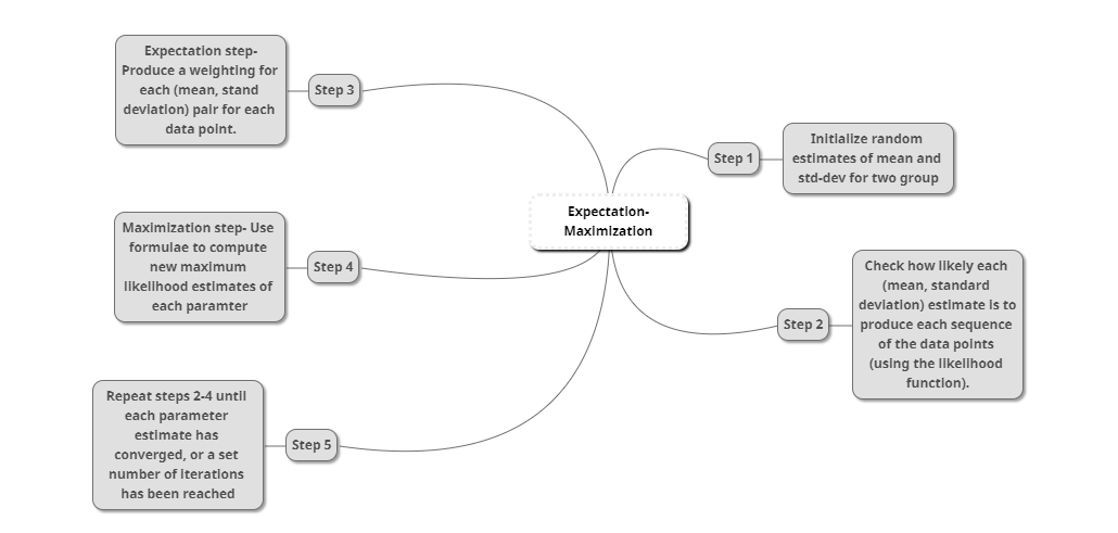
Since we already have the likelihood function from our stats module we only need to create weighting,estimate_mean and estimate_std function
def weight_of_colour(colour_likelihood, total_likelihood):
    """
    Compute the weight for each colour at each data point.
    """
    return colour_likelihood / total_likelihood
def estimate_mean(data, weight):
    """
    For each data point, multiply the point by the probability it
    was drawn from the colour's distribution (its "weight").

    Divide by the total weight: essentially, we're finding where
    the weight is centred among our data points.
    """
    return np.sum(data * weight) / np.sum(weight)
def estimate_std(data, weight, mean):
    """
    For each data point, multiply the point's squared difference
    from a mean value by the probability it was drawn from
    that distribution (its "weight").

    Divide by the total weight: essentially, we're finding where
    the weight is centred among the values for the difference of
    each data point from the mean.

    This is the estimate of the variance, take the positive square
    root to find the standard deviation.
    """
    variance = np.sum(weight * (data - mean)**2) / np.sum(weight)
    return np.sqrt(variance)
We will plot_guess function to plot guesses
from scipy import stats
def plot_guesses(red_mean_guess, blue_mean_guess, red_std_guess, blue_std_guess, alpha=1):
    """
    Plot bell curves for the red and blue distributions given guesses for mean and standard deviation.

    alpha : transparency of the plotted curve
    """
    # set figure size and plot the purple dots
    plt.rcParams['figure.figsize'] = (15, 5)
    plt.plot(both_colours, np.zeros_like(both_colours), '.', color='purple', markersize=10)

    # compute the size of the x axis
    lo = np.floor(both_colours.min()) - 1
    hi = np.ceil(both_colours.max()) + 1
    x = np.linspace(lo, hi, 500)

    # plot the bell curves
    plt.plot(x, stats.norm(red_mean_guess, red_std_guess).pdf(x), color='r', alpha=alpha)
    plt.plot(x, stats.norm(blue_mean_guess, blue_std_guess).pdf(x), color='b', alpha=alpha)

    # vertical dotted lines for the mean of each colour - find the height
    # first (i.e. the probability of the mean of the colour group)
    r_height = stats.norm(red_mean_guess, red_std_guess).pdf(red_mean_guess)
    b_height = stats.norm(blue_mean_guess, blue_std_guess).pdf(blue_mean_guess)

    plt.vlines(red_mean_guess, 0, r_height, 'r', '--', alpha=alpha)
    plt.vlines(blue_mean_guess, 0, b_height, 'b', '--', alpha=alpha);
Let's start with EM algorithm and see how it converges to almost actual mean and std-dev of two sample group
Step 1: Start with initial random guess
# estimates for red group
red_mean_guess = 1.1
red_std_guess = 2

# estimates for blue group
blue_mean_guess = 9
blue_std_guess = 1.7

plot_guesses(red_mean_guess, blue_mean_guess, red_std_guess, blue_std_guess)

we can clearly see these guesses are not good. We knew that each group had an equal number of points, but the mean of each distribution looks to be far off any possible "middle"value.
Let's perform 15 iterations of Expectation Maximisation to improve these estimates:
N_ITER = 15 # number of iterations of EM

alphas = np.linspace(0.2, 1, N_ITER) # transparency of curves to plot for each iteration


# plot initial estimates
plot_guesses(red_mean_guess, blue_mean_guess, red_std_guess, blue_std_guess, alpha=0.13)


for i in range(N_ITER):

    ##Step 2 : Likelihood function
    likelihood_of_red = stats.norm(red_mean_guess, red_std_guess).pdf(both_colours)
    likelihood_of_blue = stats.norm(blue_mean_guess, blue_std_guess).pdf(both_colours)

    #Step 3
    ## Expectation step
    ## ----------------

    red_weight = weight_of_colour(likelihood_of_red, likelihood_of_red+likelihood_of_blue)
    blue_weight = weight_of_colour(likelihood_of_blue, likelihood_of_red+likelihood_of_blue)

    #Step 4
    ## Maximization step
    ## -----------------

    # N.B. it should not ultimately matter if compute the new standard deviation guess
    # before or after the new mean guess

    red_std_guess = estimate_std(both_colours, red_weight, red_mean_guess)
    blue_std_guess = estimate_std(both_colours, blue_weight, blue_mean_guess)

    red_mean_guess = estimate_mean(both_colours, red_weight)
    blue_mean_guess = estimate_mean(both_colours, blue_weight)

    plot_guesses(red_mean_guess, blue_mean_guess, red_std_guess, blue_std_guess, alpha=alphas[i])

plt.title(
    r'Estimates of group distributions after {} iterations of Expectation Maximisation'.format(
        N_ITER
    ),
    fontsize=17);
    #Step 5: for loop repeats step 2-4 for N_ITER

You should be able to see the shape of each bell curve converging. Let's compare our estimates to the true values for mean and standard deviation:
from IPython.display import Markdown

md = """
|            | True Mean      | Estimated Mean | True Std.      | Estimated Std. |
| :--------- |:--------------:| :------------: |:-------------: |:-------------: |
| Red        | {true_r_m:.3f} | {est_r_m:.3f}  | {true_r_s:.3f} | {est_r_s:.3f}  |
| Blue       | {true_b_m:.3f} | {est_b_m:.3f}  | {true_b_s:.3f} | {est_b_s:.3f}  |
"""

Markdown(
    md.format(
        true_r_m=np.mean(red),
        true_b_m=np.mean(blue),

        est_r_m=red_mean_guess,
        est_b_m=blue_mean_guess,

        true_r_s=np.std(red),
        true_b_s=np.std(blue),

        est_r_s=red_std_guess,
        est_b_s=blue_std_guess,
    )
)
estimate_mean() and estimate_std() were most crucial function and how weights are assigned to each data point is key to whole EM algorithm